
1D Ising Model Solution
Published:
Famously, the 1D Ising model has no phase transition when varying a magnetic field in the parallel direction. Here we will show how that is analytically derived, and develop some mathematical techniques along the way.
Transfer Matrices
We will first do this for the case of 0 field. The Hamiltonian of the 1D Ising model with no field is $H = \sum_i J S_i S_{i+1}$. Then, our partition function is
\[Z = \sum_{\{S_i\}}e^{\beta ( \sum_i J S_i S_{i+1})}.\]We will fix boundary conditions such that they are fixed and $S_0 = S_N $. Then, the smallest chain we can have is when $N = 2$.
\[Z = \sum_{S_0}\sum_{S_1}e^{\beta JS_0 S_1} = 2e^{\beta J} + 2e^{-\beta J}.\]Notice that we have a sum over both $S_0$ and $S_1$ here. Since each $S_i \in {+1,-1}$, we can identify the two values with the two basis states of a spin 1/2 system. Suppose we wrote this in the following way.
$ Z = \sum_{S_0}\sum_{S_1}\langle S_0| \begin{pmatrix} e^{\beta J} & e^{-\beta J} \ e^{-\beta J} & e^{\beta J} \end{pmatrix} |S_1\rangle. $
If
\[|S_i\rangle \in \begin{pmatrix} 1 \\ 0 \end{pmatrix}, \begin{pmatrix} 0 \\ 1 \end{pmatrix},\]then this equals what we had above. The elements of the matrix were determined by considering the terms in the summation that came from the possible combinations of $S_0,S_1$. For instance, the top-left element is the term in the partition function corresponding to when both $S_0,S_1$ are pointed up. What about for $N=3$?
\[Z = \sum_{S_0}\sum_{S_1}\sum_{S_2}e^{\beta JS_0 S_1}e^{\beta JS_1 S_2} e^{\beta JS_2 S_0}.\]After carrying out this summation (using Mathematica :D ) we get
\[Z = 6 e^{-\beta J}+2 e^{3 \beta J}.\]However, can we do the same thing as before?
\[Z = \sum_{S_0}\sum_{S_1}\sum_{S_2}\langle S_0| \begin{pmatrix} e^{\beta J} & e^{-\beta J} \\ e^{-\beta J} & e^{\beta J} \end{pmatrix}| S_1\rangle \langle S_1| \begin{pmatrix} e^{\beta J} & e^{-\beta J} \\ e^{-\beta J} & e^{\beta J} \end{pmatrix}|S_2 \rangle \langle S_2| \begin{pmatrix} e^{\beta J} & e^{-\beta J} \\ e^{-\beta J} & e^{\beta J} \end{pmatrix}| S_0 \rangle.\]Notice that if we carry out the sum over $S_1$, we get
\[\sum_{S_1}|S_1\rangle\langle S_1| = \begin{pmatrix} 1 & 0 \\ 0 & 1 \end{pmatrix},\]which is the identity matrix. The same thing occurs for $S_2$. We can simplify the partition function then to
\[Z = \sum_{S_0}\langle S_0| \begin{pmatrix} e^{\beta J} & e^{-\beta J} \\ e^{-\beta J} & e^{\beta J} \end{pmatrix} ^ 2| S_0 \rangle = Tr \begin{pmatrix} e^{\beta J} & e^{-\beta J} \\ e^{-\beta J} & e^{\beta J} \end{pmatrix} ^ 2 = 6 e^{-\beta J}+2 e^{3 \beta J}.\]It agrees with the direct summation. This should work for any $N$ spins. The matrix that we introduced is called a transfer matrix. The reason this can be done this way is because every spin is contained between only two terms in the Hamiltonian, and so the sum over any given spin can be re-written as a repeated index summation on a product of matrices. The transfer matrix between spins $i,i+1$ is
\[T = \begin{pmatrix} e^{\beta J} & e^{-\beta J} \\ e^{-\beta J} & e^{\beta J} \end{pmatrix}.\]It defines all possible interaction terms in the partition function between the two spins.
We can extend this analysis to when we have a parallel field. In that case our Hamiltonian becomes
\[H = \sum_i J S_i S_{i+1} + h S_i.\]For $N=2$, we have the partition function
\(Z = \sum_{S_0}\sum_{S_1}e^{\beta JS_0 S_1 + \beta hS_0 + \beta h S_1}\) \(=\sum_{S_0}e^{\beta J S_0 + \beta h S_0 + \beta h} + e^{-\beta J S_0 + \beta h S_0 -\beta h}\) \(=e^{\beta J + \beta h + \beta h} + e^{-\beta J - \beta h + \beta h} + e^{-\beta J + \beta h -\beta h} + e^{\beta J - \beta h -\beta h}\) $$=e^{\beta J}(e^{2\beta h} + e^{-2\beta h}) +2e^{-\beta J}$.
Our goal again is to write this as a sum over the elements of a matrix. The natural starting point is to consider a modification to our original transfer matrix. Recall that we are considering a field parallel to our Ising spins, and we mapped our spins to the states of a spin 1/2 system. Moreover, consider the form of the partition function for only fields and no interactions.
\[Z = \sum_{S_0}\sum_{S_1}e^{\beta hS_0 + \beta h S_1} =e^{\beta h + \beta h} + e^{\beta h-\beta h }+e^{-\beta h+\beta h } + e^{-\beta h - \beta h} = e^{2 \beta h}+e^{-2 \beta h}.\]To write this in bra-ket notation with a matrix as before, we can do
\[Z = \sum_{S_0}\sum_{S_1} \langle S_0| \begin{pmatrix} e^{2\beta h} & 0 \\ 0 & e^{-2\beta h} \end{pmatrix} |S_1 \rangle.\]Combining this with the Ising interaction transfer matrix we get
\[T= \begin{pmatrix} e^{\beta J + 2\beta h} & e^{-\beta J} \\ e^{-\beta J} & e^{\beta J - 2\beta h} \end{pmatrix}.\]Again this comes from considering the terms in the partition function which correspond to the particular spin configurations. The top-left is when both spins are pointed upwards, top right, when $S_0$ is up and $S_1$ is down, and so on. As expected, summing the matrix elements of this, yields the correct partition function $N = 2$.
However, one has to be careful when going beyond two spins. The reason is, $T$ encapsulates all the terms in the Hamiltonian corresponding to $S_i,S_{i+1}$. However, the field interaction term for $S_{i+1}$ will appear in $T_{i,i+1},\ T_{i+1,i+2}$, naively multiplying $T$ repeatedly to get the full partition function will cause us to double count. The solution to this is to separate out the field interaction terms by writing $T$ as a matrix product.
\[T = T_H T_J T_H = \begin{pmatrix} e^{\beta h} & 0 \\ 0 & e^{-\beta h} \end{pmatrix} \begin{pmatrix} e^{\beta J } & e^{-\beta J} \\ e^{-\beta J} & e^{\beta J} \end{pmatrix} \begin{pmatrix} e^{\beta h} & 0 \\ 0 & e^{-\beta h} \end{pmatrix}.\]Then, what we can do is write a modified transfer matrix that has $T_H \to T_H^{1/2}$ such that upon repeated multiplication, we will only pick up one factor of $T_H$ per spin.
\[T' =T_H^{1/2} T_J T_H^{1/2}= \begin{pmatrix} e^{\beta J + \beta h} & e^{-\beta J} \\ e^{-\beta J} & e^{\beta J - \beta h} \end{pmatrix}.\]Now, our full partition function for $N$ spins can be written as
\[Z = \sum_{S_0}\langle S_0|T'^N |S_0\rangle = Tr[T'^N].\]To get an expression for $Z$, we need two facts. The first is that the trace is a sum over eigenvalues. The second is $Tr[AB]=Tr[A]Tr[B]$. That means
\[Z = \lambda_+^N + \lambda_-^N,\]where $\lambda_+,\lambda_-$ are the two eigenvalues of $T’$. The eigenvalues of $T’$ are
\[\lambda_{\pm}=\frac{1}{2} e^{\beta J-\beta h}+\frac{1}{2} e^{\beta h+\beta J}\pm\frac{1}{2} e^{\beta (-h)-\beta J} \sqrt{4 e^{2 \beta h}-2 e^{2 \beta h+4 \beta J}+e^{4 \beta h+4 \beta J}+e^{4 \beta J}}.\]Obtained from Mathematica, but we could simplify this:
\[\lambda_{\pm}=e^{\beta J}\cosh \beta h \pm \frac{1}{2}e^{-\beta h - \beta J}\sqrt{e^{4\beta J}(1 - e^{2\beta h} )^2 + 4e^{2\beta h}}.\]Great so now we have some expression for the partition function. It is the sum of each of the eigenvalues to the $N$th power.
Expectation Values
Now, suppose we wanted to calculate the expectation value of some quantity, say spin $i$. We know that from statistical mechanics, this quantity is
\[\langle S_i \rangle= \frac{\sum_{S_0} \sum_{S_1} ... \sum_{S_i} ... S_i e^{\beta J \sum_{j}S_j S_{j+1} + \beta h \sum_j S_j}}{Z}.\]For the sake of tractability, let’s first just do this for $N=3$ and ask about $\langle S_1 \rangle$.
\[\langle S_1 \rangle= \frac{\sum_{S_0} \sum_{S_1} \sum_{S_2} S_1 e^{\beta J (S_0 S_1 + S_1 S_2 + S_2 S_0 + \beta h (S_0 + S_1 +S_2)}}{Z}.\]We can write the numerator in bra-ket notation as before.
\[\langle S_1 \rangle= \frac{\sum_{S_0} \sum_{S_1} \sum_{S_2} S_1 \langle S_0|T'|S_1\rangle \langle S_1| T'|S_2 \rangle \langle S_2| T' |S_0 \rangle}{Z} .\]Notice now however, that when we do the sum over $S_1$, we don’t simply get the identity. We have to multiply the value in the sum by the value of $S_1$. That means the term in the sum which corresponds to “down-spin” must pick up a minus sign. $S_1$ is a scalar so we were allowed to move it through the transfer matrices without worrying about commutation relations. We can move the $S_1$ through the expression to obtain
\[\langle S_1 \rangle= \frac{\sum_{S_0} \sum_{S_1} \sum_{S_2} \langle S_0|T' S_1 |S_1\rangle \langle S_1| T'|S_2 \rangle \langle S_2| T' |S_0 \rangle}{Z}.\]This sort of looks like a spin operator acting on a state. In fact, now when we perform the summation over $S_1$, we get
\[\sum_{S_1}S_1|S_1\rangle \langle S_1| = +1 \begin{pmatrix} 1 & 0\\ 0 & 0 \end{pmatrix} -1 \begin{pmatrix} 0 & 0\\ 0 & 1 \end{pmatrix} = \begin{pmatrix} 1 & 0\\ 0 & -1 \end{pmatrix} = S^z.\]Evidently, the expectation value of $S_1$ can be expressed simply through inserting an $S^z$ into the appropriate slot in the product in the numerator. We have then, for an $N$ spin system,
\[\langle S_i \rangle=\frac{\sum_{S_0}\langle S_0|T'^{i-1} S^z_i T'^{N-i - 1} |S_0\rangle}{Z} = \frac{Tr[T'^{i-1} S^z_i T'^{N-i - 1}]}{Z}.\]Similarly, we can calculate spin-spin correlation functions.
\[\langle S_i S_j\rangle=\frac{\sum_{S_0}\langle S_0|T'^{i-1} S^z_i T'^{j- i }S^z_j T^{N-j+1} |S_0\rangle}{Z} = \frac{Tr[T'^{i-1} S^z_i T'^{j- i }S^z_j T^{N-j+1} ]}{Z}.\]Suppose we now wanted to actually calculate one of these quantities. Let’s look at the correlation length. We know that due to translation symmetry, every one of the transfer matrices are the same. The transfer matrices are diagonalizable and therefore there are unitary operations which rotate the transfer matrices into their eigenbasis. These unitary operators are of course the matrix of eigenvectors of $T’$.We can rewrite the trace using
\[Tr[UU^{-1}TUU^{-1}T...TUU^{-1} S^z UU^{-1} T'...T'UU^{-1} S^z UU^{-1} T...TUU^{-1} ] = Tr[U \begin{pmatrix} \lambda_+^{i-1} & 0 \\ 0 & \lambda_-^{i-1} \end{pmatrix}U^{-1}S^zU \begin{pmatrix} \lambda_+^{j-i} & 0 \\ 0 & \lambda_-^{j-i} \end{pmatrix}U^{-1}S^zU \begin{pmatrix} \lambda_+^{N-j+1} & 0 \\ 0 & \lambda_-^{N-j+1} \end{pmatrix}U^{-1}].\]What is the matrix $U$?
\[U = \begin{pmatrix} -\frac{1}{2} e^{\beta (-h)} \sqrt{4 e^{2 \beta h}-2 e^{2 \beta h+4 \ \beta J}+e^{4 \beta h+4 \beta J}+e^{4 \beta J}}-\frac{1}{2} e^{2 \ \beta J-\beta h}+\frac{1}{2} e^{\beta h+2 \beta J} & \frac{1}{2} e^{\beta (-h)} \sqrt{4 e^{2 \beta h}-2 e^{2 \beta h+4 \ \beta J}+e^{4 \beta h+4 \beta J}+e^{4 \beta J}}-\frac{1}{2} e^{2 \ \beta J-\beta h}+\frac{1}{2} e^{\beta h+2 \beta J} \\ 1 & 1 \end{pmatrix}.\]Of course, since this is a unitary matrix, it can be written in the form
\[U = \begin{pmatrix} e^{i(\alpha -\beta / 2 -\delta / 2)}\cos \frac{\gamma}{2} & -e^{i(\alpha -\beta / 2 +\delta / 2)}\sin \frac{\gamma}{2} \\ e^{i(\alpha +\beta / 2 -\delta / 2)}\sin \frac{\gamma}{2} & e^{i(\alpha +\beta / 2 +\delta / 2)}\cos \frac{\gamma}{2} \end{pmatrix}.\]This has the inverse:
\[U^{-1} = \begin{pmatrix} e^{-\frac{1}{2} i (2 \alpha \ -\beta -\delta )}\cos \frac{\gamma }{2} &e^{-\frac{1}{2} i (2 \alpha +\beta -\delta )} \sin \frac{\gamma }{2} \ \\ -e^{-\frac{1}{2} i (2 \ \alpha -\beta +\delta )} \sin \frac{\gamma }{2} & e^{-\frac{1}{2} i (2 \alpha +\beta +\delta )} \cos \frac{\gamma }{2} \end{pmatrix}.\]The trace becomes
\[Tr[ \begin{pmatrix} e^{i(\alpha -\beta / 2 -\delta / 2)}\cos \frac{\gamma}{2} & -e^{i(\alpha -\beta / 2 +\delta / 2)}\sin \frac{\gamma}{2} \\ e^{i(\alpha +\beta / 2 -\delta / 2)}\sin \frac{\gamma}{2} & e^{i(\alpha +\beta / 2 +\delta / 2)}\cos \frac{\gamma}{2} \end{pmatrix} \begin{pmatrix} \lambda_+^{i-1} & 0 \\ 0 & \lambda_-^{i-1} \end{pmatrix} \begin{pmatrix} \cos (\gamma ) & -e^{i \delta } \sin (\gamma ) \\ -e^{-i \delta } \sin (\gamma ) & -\cos (\gamma ) \end{pmatrix} \begin{pmatrix} \lambda_+^{j-i} & 0 \\ 0 & \lambda_-^{j-i} \end{pmatrix} \begin{pmatrix} \cos (\gamma ) & -e^{i \delta } \sin (\gamma ) \\ -e^{-i \delta } \sin (\gamma ) & -\cos (\gamma ) \end{pmatrix} \begin{pmatrix} \lambda_+^{N-j+1} & 0 \\ 0 & \lambda_-^{N-j+1} \end{pmatrix} \begin{pmatrix} e^{-\frac{1}{2} i (2 \alpha \ -\beta -\delta )}\cos \frac{\gamma }{2} &e^{-\frac{1}{2} i (2 \alpha +\beta -\delta )} \sin \frac{\gamma }{2} \ \\ -e^{-\frac{1}{2} i (2 \ \alpha -\beta +\delta )} \sin \frac{\gamma }{2} & e^{-\frac{1}{2} i (2 \alpha +\beta +\delta )} \cos \frac{\gamma }{2} \end{pmatrix}].\]This looks terrible but we can make a few inroads though. Due to the cyclic property of the trace, we can write
\[Tr[UT_r'^{i-1}U^{-1}S^zUT_r'^{j-i}U^{-1}S^zUT_r'^{N-j+1}U^{-1}] = Tr[U^{-1}UT_r'^{i-1}U^{-1}S^zUT_r'^{j-i}U^{-1}S^zUT_r'^{N-j+1}] = Tr[T_r'^{i-1}U^{-1}S^zUT_r'^{j-i}U^{-1}S^zUT_r'^{N-j+1}].\]Written out using matrices, we have
\[Tr[ \begin{pmatrix} \lambda_+^{i-1} & 0 \\ 0 & \lambda_-^{i-1} \end{pmatrix} \begin{pmatrix} \cos (\gamma ) & -e^{i \delta } \sin (\gamma ) \\ -e^{-i \delta } \sin (\gamma ) & -\cos (\gamma ) \end{pmatrix} \begin{pmatrix} \lambda_+^{j-i} & 0 \\ 0 & \lambda_-^{j-i} \end{pmatrix} \begin{pmatrix} \cos (\gamma ) & -e^{i \delta } \sin (\gamma ) \\ -e^{-i \delta } \sin (\gamma ) & -\cos (\gamma ) \end{pmatrix} \begin{pmatrix} \lambda_+^{N-j+1} & 0 \\ 0 & \lambda_-^{N-j+1} \end{pmatrix}].\]Again using the cyclic trace property:
\[Tr[ \begin{pmatrix} \lambda_+^{N-j + i} & 0 \\ 0 & \lambda_-^{N-j + i} \end{pmatrix} \begin{pmatrix} \cos (\gamma ) & -e^{i \delta } \sin (\gamma ) \\ -e^{-i \delta } \sin (\gamma ) & -\cos (\gamma ) \end{pmatrix} \begin{pmatrix} \lambda_+^{j-i} & 0 \\ 0 & \lambda_-^{j-i} \end{pmatrix} \begin{pmatrix} \cos (\gamma ) & -e^{i \delta } \sin (\gamma ) \\ -e^{-i \delta } \sin (\gamma ) & -\cos (\gamma ) \end{pmatrix} ].\]Now we can carry out the matrix multiplication.
\[Tr[ \begin{pmatrix} \lambda _+^N (\cos ^2(\gamma )+\sin ^2(\gamma ) \lambda _-^{j-i} \lambda _+^{i-j}) & e^{i \delta } \sin (\gamma ) \cos \ (\gamma ) \lambda _+^N (\lambda _+^{i-j} \lambda_-^{j-i}-1 \\ e^{-i \delta } \sin (\gamma ) \cos (\gamma ) \lambda _ -^N \ (1-\lambda _+^{j-i} \lambda _-^{i-j}) & \lambda _-^N \ (\cos ^2(\gamma )+\sin ^2(\gamma ) \lambda _+^{j-i} \lambda _-^{i-j}) \end{pmatrix}]\] \[= \lambda _+^N (\cos ^2(\gamma )+\sin ^2(\gamma ) \lambda _-^{j-i} \lambda _+^{i-j}) + \lambda _-^N \ (\cos ^2(\gamma )+\sin ^2(\gamma ) \lambda _+^{j-i} \lambda _-^{i-j}) =\cos ^2(\gamma )(\lambda_+^N + \lambda_-^N) + \sin ^2(\gamma )\left( \lambda_+^N\left( \frac{\lambda_+}{\lambda_-}\right)^{i-j}+\lambda_-^N\left( \frac{\lambda_+}{\lambda_-}\right)^{j-i} \right).\]There we go. Then finally, we can write the spin-spin correlation function as
\[\langle S_i S_j\rangle = \frac{\cos ^2(\gamma )(\lambda_+^N + \lambda_-^N) + \sin ^2(\gamma )\left( \lambda_+^N\left( \frac{\lambda_+}{\lambda_-}\right)^{i-j}+\lambda_-^N\left( \frac{\lambda_+}{\lambda_-}\right)^{j-i} \right)}{\lambda_+^N+\lambda_-^N}.\]We can make some simplications.
\[\langle S_i S_j\rangle = \cos^2\gamma + \sin^2\gamma \left(\frac{\lambda_+^{N+i-j}\lambda_-^{j-i}+\lambda_-^{N+i-j}\lambda_+^{j-i}}{\lambda_+^N+\lambda_-^N} \right)\] \[=\cos^2\gamma + \sin^2\gamma \left(\frac{\left(\frac{\lambda_+}{\lambda_-}\right)^{N+i-j}+\left(\frac{\lambda_-}{\lambda_+}\right)^{i-j}}{\left(\frac{\lambda_+}{\lambda_-}\right)^N+1} \right).\]Let’s examine the behavior of the eigenvalues as $N \to \infty$.
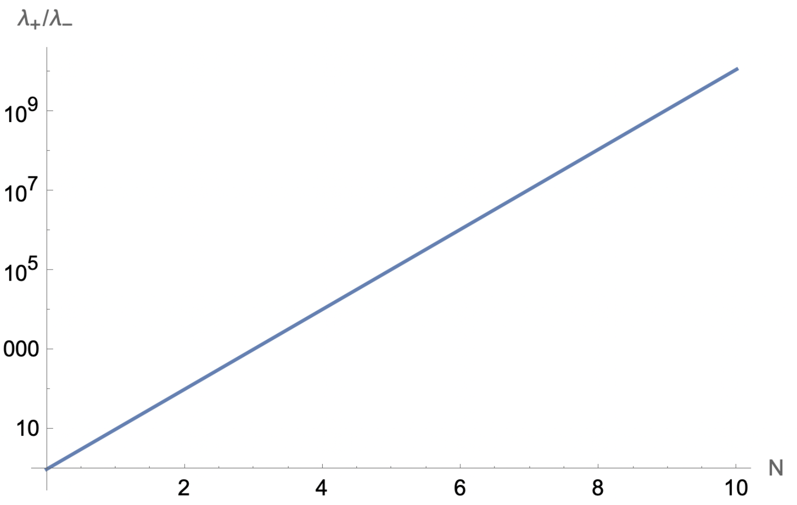
Evidently, only the largest eigenvalue matters. This allows us to simplify the trace above.
\[\approx\cos^2\gamma + \sin^2\gamma \left(\frac{\left(\frac{\lambda_+}{\lambda_-}\right)^{N+i-j}}{\left(\frac{\lambda_+}{\lambda_-}\right)^N} \right)\] \[=\cos^2\gamma + \sin^2\gamma \left(\frac{\lambda_+}{\lambda_-}\right)^{i-j} .\]In the termodynamic limit, this is the spin-spin correlation function.
Phase Transitions
The partition function and its derivative thermodynamic quantities are all smooth functions of their arguments except at critical points. At critical points (i.e. where a phase transition occurs), these quantities and/or their derivatives are non-analytic. By non-analytic, I mean the functions have some kind of abrupt change, like a kink, or jump discontinuity.
There are two types of *thermal *phase transitions: first order phase transitions and continuous phase transitions.
1) First Order phase transitions: In first order phase transitions, a latent heat is involved. The temperature stays constant as heat is added and there is phase coexistence. The free energy ($\sim \ln Z$) at the critical point of a first-order phase transition is continuous but has a “kink” such that the first derivative and beyond of the free energy, have discontinuities. The first derivative of the free energy, the internal energy, has a jump discontinuity corresponding to the latent heat. 2) Continuous phase transitions: Continuous phase transitions are characterized by some kind of diverging thermodynamic quantity, like the correlation length. They come from places where higher order derivatives of the free energy diverge. The first derivative of the free energy (and therefore the internal energy) is continuous but the second derivative has a singularity.
There is a pretty good stack exchange thread on this that has some pictures which I learned from (https://physics.stackexchange.com/questions/80245/first-and-second-order-phase-transitions). Anyway the point is, in the 1D Ising model, our free energy isn’t some piece wise defined thing. So that rules out first order phase transitions. Our goal then is to look for places where the higher order derivatives of the free energy with respect to $\beta$ diverges.
The free energy in the thermodynamic limit is
\[F = -\frac{1}{\beta} \ln Z = -\frac{1}{\beta} \ln \lambda_+^N.\]The internal energy is
\[E = \frac{d (\beta F)}{d \beta} = \frac{d \ln Z}{d\beta} = -\frac{d}{d\beta} \ln \lambda_+^N = -\frac{1}{\lambda_+^N} N \lambda_+^{N-1} \frac{d}{d\beta} \lambda_+.\]This is a horribly nasty expression, but we can plot this in Mathematica.

We see here that the second derivative of the energy is in fact not singular for any $\beta$ at these different values for $h$. This is indicative of a lack of a phase transition in the 1D Ising model, regardless of applied field. We can see this ourselves. Let’s set $h=0$ in all of our expressions above. First, the free energy.
\[F = -\frac{1}{\beta}\ln (2\cosh \beta J)^N.\]The internal energy is then
\[E = \frac{d (\beta F)}{d \beta} = NJ \tanh \beta J.\]This has no singularity for any $\beta > 0$. Now the spin-spin correlation function.
\[\langle S_i S_j\rangle =\left(\frac{\lambda_+}{\lambda_-}\right)^{|i-j|} = (\tanh \beta J)^{|i-j|}.\]We can rewrite this as an exponential.
\[\exp(\ln (\tanh \beta J)^{|i-j|}) = \exp(|i-j|\ln (\tanh \beta J)) = \exp \left[ \frac{|i-j|}{1 / \ln (\tanh \beta J)} \right].\]The correlation length, defined by
\[\xi = 1 / \ln (\tanh \beta J).\]is finite for any $\beta > 0$.
Notice that $\tanh \beta J < 1$ for any $\beta$ so the above expression indicates exponential decay with increasing separation.
We have that for any finite temperature, there is no phase transition at 0 field. And as we stated above, for any finite field, the free energy is analytic. So there is no phase transition for any field and for any temperature. But what is the phase?
This we can figure out using an order parameter. We shall use the overall magnetization
\[\langle m \rangle =\langle \sum_i S_i \rangle.\]Using the partition function,
\[\langle m \rangle = \frac{\sum_{S_0} \sum_{S_1} ... \sum_{S_i} ... \left(\sum_i S_i \right) e^{\beta J \sum_{j}S_j S_{j+1} + \beta h \sum_j S_j}}{Z} = \frac{\sum_i \langle S_i \rangle}{Z} = \frac{\sum_i Tr \left[ \begin{pmatrix} \lambda_+^{i-1} & 0 \\ 0 & \lambda_-^{i-1} \end{pmatrix} \begin{pmatrix} \cos (\gamma ) & -e^{i \delta } \sin (\gamma ) \\ -e^{-i \delta } \sin (\gamma ) & -\cos (\gamma ) \end{pmatrix} \begin{pmatrix} \lambda_+^{N-i} & 0 \\ 0 & \lambda_-^{N-i} \end{pmatrix}\right]}{Z}=\frac{\sum_i Tr \left[ \begin{pmatrix} \lambda_+^{N-1} & 0 \\ 0 & \lambda_-^{N-1} \end{pmatrix} \begin{pmatrix} \cos (\gamma ) & -e^{i \delta } \sin (\gamma ) \\ -e^{-i \delta } \sin (\gamma ) & -\cos (\gamma ) \end{pmatrix} \right]}{Z}\] \[= \frac{\sum_i (\lambda_+^{N-1} + \lambda_-^{N-1})\cos \gamma}{Z} = \frac{N(\lambda_+^{N-1} + \lambda_-^{N-1})\cos \gamma}{Z} = \frac{N(\lambda_+^{N-1} + \lambda_-^{N-1})\cos \gamma}{\lambda_+^N + \lambda_-^N}.\]$N-1\approx N$ in the thermodynamic limit so we can cancel terms. We’re left with
\[\langle m \rangle = N\cos \gamma.\]Recall the definition of $\gamma$. $\gamma$ is the rotation in the unitary which we apply in order to diagonalize the transfer matrix. When $\gamma=0$, $U$ is diagonal, meaning the interaction term is 0 and the only term present is the field. We can take $\gamma \to 0$ to be the limit where the field is so much stronger than the interaction that the ratio $h/J \to \infty$. When $\gamma = 0$, we see that the system is completely magnetized. When $\gamma = \pi/2$, the system has 0 magnetization and is completely disordered. From this, we can deduce that the phase is paramagnetic.
Through the transfer matrix technique, we have shown that the 1D Ising model has no phase transition and is a paramagnet for any temperature and parallel field.